sentinel-1/2
哨兵2号
哨兵 2 号共有 13 个波段,目前有 2 颗卫星,第一颗卫星 Sentinel 2A 2015年发射,第二颗 Sentinel 2B 2017年发射,后续 Sentinel 2C, Sentinel 2D 将于 2024年发射,这样将有 4 颗哨兵 2 号卫星,后续发射的卫星将提高一倍哨兵 2 号的重坊周期。
波段介绍
哨兵二号装载多光谱成像仪,传感器共有 13 个波段,空间分辨率从 10m 到 60m 都有。
- 蓝(B2)、绿(B3)、红(B4)和近红外(B8)波段,空间分辨率为 10m
- 红边(B5)、近红外(B6, B7, B8A)、和短波红外(B11, B12),空间分辨率为 20m
- 海岸带/气溶胶(B1)、卷云波段(B10),空间分辨率 60m
波段组合
- 真彩色(4,3,2)
- 假彩色(8,4,3)
If you want to see Sentinel band combinations for yourself, you can check out the Sentinel Playground. It visualizes the band combinations below, as well as several more.
参考文献: - GISGeography
- Sentinel Playground
哨兵1号
哨兵1号sentinel-1 由两颗极轨卫星A星和B星组成。两颗卫星搭载的传感器为合成孔径雷达(SAR),属于主动微波遥感卫星。传感器搭载C波段。
哨兵1号的条带扫描模式
SM(Stripmap):一种标准的SAR条形图成像模式,其中地面区域被连续的脉冲序列照亮,而天线波束指向一个固定的方位角和仰角。
SM模式仅用于小岛屿,在紧急情况管理等特殊事件时使用。- L0 RAW
- L1 SLC
- L1 GRD (Full resolution, High resolution, Medium resolution)
IW(Interferometric Wide swath):IW)模式是陆地上的主要采集模式,满足了大部分业务需求。它以5米 x 20米的空间分辨率(单视)获取250公里长的数据。IW模式使用渐进扫描SAR (TOPSAR)地形观测捕获三个子区域。在TOPSAR技术中,除了像扫描雷达一样控制波束的范围外,波束还可以在每个爆发的方位角方向上由后向前进行电子控制,避免了扇形现象,并导致整个区域的图像质量均匀。
- L0 RAW
- L1 SLC
- L1 GRD (High resolution, Medium resolution)
EW(Extra Wide swath):使用TOPSAR成像技术在五个区域获取数据。EW模式以牺牲空间分辨率为代价提供了非常大的区域覆盖。(言外之意是空间分辨率低)。
EW模式主要用于沿海监测,包括海运监测、溢油监测和海冰监测。- L0 RAW
- L1 SLC
- L1 GRD (High resolution, Medium resolution)
WV(Wave): 数据是在被称为“小片段”的小型条形地图场景中获取的,这些场景在轨道沿线每隔100公里定期设置一次。通过交替获得小点,以近距离入射角获得一个小点,而以远距离入射角获得下一个小点。WV是哨兵1号在海上的操作模式。(言外之意用于
海洋)。- L1 SLC
- L2 OCN (OSW RVL)
对于每一种模式,都可以生产SAR的0级、1级SLC、1级GRD 和2级OCN的产品。
哨兵1号的数据产品
- Raw Level-0 data (特定情况下使用)
- SLC( Single Look Complex):已被处理后的一级产品,能获得相位和振幅信息。相位信息是时间的函数,根据相位信息和速度可实现距离的测量。(可用于
测距和形变观测)。 - GRD(Ground Range Detected):一级产品,有多视强度数据,该强度数据与后向散射系数有关。(可用于
土壤水分反演)。 - OCN(Ocean):用于检索海洋地球物理参数。(即应用于
海洋)。
所有的产品都是从0级产品直接加工的。每种模式都可以潜在地生成一级SLC、一级GRD和二级Ocean产品
应用
- 海上监测(Maritime monitoring)
- Land monitoring
- Energency management
- Mapping applications to sentinel-1 modes
极化方式
- 单极化方式: HH 或 VV
- 双极化方式: HH+HV 或 VV+VH
WV扫描模式只有单极化方式HH或VV。其他扫描模式单极化方式(HH或VV)和双极化方式(HH+HV或VV+VH)都有。
IW:用(VV+VH)极化方式–>观测陆地;
WV: 用VV极化方式–>观测海洋.
参考文献:塞翁的读书笔记
哨兵1号分辨率
- SLC 1级产品分辨率
| mode | resolution(rgxaz) | pixel spacing(rgxaz) | number of looks | enl |
|---|---|---|---|---|
| SM | 1.7X4.3m to 3.6x4.9m | 1.5x3.6m to 3.1x4.1m | 1x1 | 1 |
| IW | 2.7x22m to 3.5x22m | 2.3x14.1m | 1x1 | 1 |
| EW | 7.9X43m to 15x43m | 5.9x19.9m | 1x1 | 1 |
| WV | 2.0X4.8m and 3.1x4.8m | 1.7x4.1m and 2.7x4.1m | 1x1 | 1 |
- GRD 1级产品分辨率
Full resolution level-1 GRD
| mode | resolution(rgxaz) | pixel spacing(rgxaz) | number of looks | enl |
|---|---|---|---|---|
| SM | 9X9m | 3.5x3.5m | 2x2 | 3.7 |
High resolution level-1 GRD
| mode | resolution(rgxaz) | pixel spacing(rgxaz) | number of looks | enl |
|---|---|---|---|---|
| SM | 23X23m | 10x10m | 6x6 | 29.7 |
| IW | 20X22m | 10x10m | 5x1 | 4.4 |
| EW | 50x50m | 25x25m | 3x1 | 2.7 |
Medium resolution level-1 GRD
| mode | resolution(rgxaz) | pixel spacing(rgxaz) | number of looks | enl |
|---|---|---|---|---|
| SM | 84X84m | 40mx40m | 22x22 | 398.4 |
| IW | 88X87m | 40x40m | 22x5 | 81.8 |
| EW | 93x87m | 40x40m | 6x2 | 10.7 |
| WV | 52x51m | 25x25m | 13x13 | 123.7 |
- 2级Ocean产品
sentinel 批量下载
环境配置
conda create -n sentinelsatsource activate sentinelsat
安装 sentinelsat 环境pip install sentinelsat
简单用法
sentinelsat -u <user> -p <password> -g <geojson>
Search and download all Sentinel-1 scenes of type SLC, in descending orbit, for the year 2015.
sentinelsat -u <user> -p <password> -g <search_polygon.geojson> -s 20150101 -e 20151231 -d --producttype SLC -q "orbitdirection=Descending" --url "https://apihub.copernicus.eu/apihub"
Username, password and DHuS URL can also be set via environment variables for convenience.
# same result as query above
export DHUS_USER="<user>"
export DHUS_PASSWORD="<password>"
export DHUS_URL="https://apihub.copernicus.eu/apihub"

sentinelsat -g <search_polygon.geojson> -s 20150101 -e 20151231 -d --producttype SLC -q "orbitdirection=Descending"
geojson 格式制作
创建 shp 转 geojson格式转换环境conda install gdal -y
转换示例ogr2ogr -f 'GeoJSON' researchArea.json researchArea.shp
参考文献:
Sentinel-2 10m LULC Time Series
为分析而优化的全球影像层。Sentinel-2 10米土地利用/土地覆盖时间序列,涵盖全球。由 Impact Observatory 和 Esri 联合制作。
描述
此图层显示了基于欧空局哨兵2号(ESA Sentinel-2)10米分辨率影像的全球土地利用/土地覆盖 (LULC) 地图。每年的地图均由 Impact Observatory’s deep learning AI land classification model 生成,该模型使用来自国家地理学会的数十亿人工标记图像像素进行训练。全球地图是通过将模型应用于 Microsoft’s Planetary Computer 的哨兵2号2A级影像集生成的,该计算机每年处理超过40万个地球观测数据。
该算法可生成九个类别的LULC地图,详见下文。
2017年的每个像素都分配了一个土地覆盖类别,但其类别划分所基于的图像数量少于其他年份。2018-2024年则基于更完整的影像集。因此,2017年的土地覆盖类别划分可能不如2018-2024年准确。
关键参数
Variable mapped: Land use/land cover in 2017, 2018, 2019, 2020, 2021, 2022, 2023, 2024
Source Data Coordinate System: Universal Transverse Mercator (UTM) WGS84
Service Coordinate System: Web Mercator Auxiliary Sphere WGS84 (EPSG:3857)
Extent: Global
Source imagery: Sentinel-2 L2A
Cell Size: 10-meters
Type: Thematic
Attribution: Esri, Impact Observatory
Analysis: Optimized for analysis
Class Definitions:
| Value | Name | Description |
|---|---|---|
| 1 | Water | Areas where water was predominantly present throughout the year; may not cover areas with sporadic or ephemeral water; contains little to no sparse vegetation, no rock outcrop nor built up features like docks; examples: rivers, ponds, lakes, oceans, flooded salt plains. |
| 2 | Trees | Any significant clustering of tall (~15 feet or higher) dense vegetation, typically with a closed or dense canopy; examples: wooded vegetation, clusters of dense tall vegetation within savannas, plantations, swamp or mangroves (dense/tall vegetation with ephemeral water or canopy too thick to detect water underneath). |
| 4 | Flooded vegetation | Areas of any type of vegetation with obvious intermixing of water throughout a majority of the year; seasonally flooded area that is a mix of grass/shrub/trees/bare ground; examples: flooded mangroves, emergent vegetation, rice paddies and other heavily irrigated and inundated agriculture. |
| 5 | Crops | Human planted/plotted cereals, grasses, and crops not at tree height; examples: corn, wheat, soy, fallow plots of structured land. |
| 7 | Built Area | Human made structures; major road and rail networks; large homogenous impervious surfaces including parking structures, office buildings and residential housing; examples: houses, dense villages / towns / cities, paved roads, asphalt. |
| 8 | Bare ground | Areas of rock or soil with very sparse to no vegetation for the entire year; large areas of sand and deserts with no to little vegetation; examples: exposed rock or soil, desert and sand dunes, dry salt flats/pans, dried lake beds, mines. |
| 9 | Snow/Ice | Large homogenous areas of permanent snow or ice, typically only in mountain areas or highest latitudes; examples: glaciers, permanent snowpack, snow fields. |
| 10 | Clouds | No land cover information due to persistent cloud cover. |
| 11 | Rangeland | Open areas covered in homogenous grasses with little to no taller vegetation; wild cereals and grasses with no obvious human plotting (i.e., not a plotted field); examples: natural meadows and fields with sparse to no tree cover, open savanna with few to no trees, parks/golf courses/lawns, pastures. Mix of small clusters of plants or single plants dispersed on a landscape that shows exposed soil or rock; scrub-filled clearings within dense forests that are clearly not taller than trees; examples: moderate to sparse cover of bushes, shrubs and tufts of grass, savannas with very sparse grasses, trees or other plants. |
NOTE: Land use focus does not provide the spatial detail of a land cover map. As such, for the built area classification, yards, parks, and groves will appear as built area rather than trees or rangeland classes.
Usage Information and Best Practices
Processing Templates
- This layer includes a number of preconfigured processing templates (raster function templates) to provide on-the-fly data rendering and class isolation for visualization and analysis.
- Each processing template includes labels and descriptions to characterize the intended usage. This may include for visualization, for analysis, or for both visualization and analysis.
Visualization
- The default rendering on this layer displays all classes.
- There are a number of on-the-fly renderings/processing templates designed specifically for data visualization.
- By default, the most recent year is displayed. To discover and isolate specific years for visualization in Map Viewer, try using the Image Collection Explorer.
Analysis
- In order to leverage the optimization for analysis, the capability must be enabled by your ArcGIS organization administrator. More information on enabling this feature can be found in the ‘Regional data hosting’ section of this help doc.
- Optimized for analysis means this layer does not have size constraints for analysis and it is recommended for multisource analysis with other layers optimized for analysis. See this group for a complete list of imagery layers optimized for analysis.
- Prior to running analysis, users should always provide some form of data selection with either a layer filter (e.g. for a specific date range, cloud cover percent, mission, etc.) or by selecting specific images. To discover and isolate specific images for analysis in Map Viewer, try using the Image Collection Explorer.
- Zonal Statistics is a common tool used for understanding the composition of a specified area by reporting the total estimates for each of the classes.
General
- If you are new to Sentinel-2 LULC, the Sentinel-2 Land Cover Explorer provides a good introductory user experience for working with this imagery layer. For more information, see this Quick Start Guide.
- Global land use/land cover maps provide information on conservation planning, food security, and hydrologic modeling, among other things. This dataset can be used to visualize land use/land cover anywhere on Earth.
Classification Process
These maps include Version 003 of the global Sentinel-2 land use/land cover data product. It is produced by a deep learning model trained using over five billion hand-labeled Sentinel-2 pixels, sampled from over 20,000 sites distributed across all major biomes of the world.
这些地图包含 Sentinel-2 全球土地利用/土地覆盖数据产品 003 版。该产品由深度学习模型生成,该模型使用超过 50 亿个手工标记的 Sentinel-2 像素进行训练,这些像素取自分布在全球所有主要生物群落的 2 万多个站点。
The underlying deep learning model uses 6-bands of Sentinel-2 L2A surface reflectance data: visible blue, green, red, near infrared, and two shortwave infrared bands. To create the final map, the model is run on multiple dates of imagery throughout the year, and the outputs are composited into a final representative map for each year.
底层深度学习模型使用 Sentinel-2 L2A 地表反射率数据的 6 个波段:可见蓝波段、绿波段、红波段、近红外波段和两个短波红外波段。为了创建最终地图,该模型会使用全年多个日期的图像运行,并将输出合成为每年的最终代表性地图。
The input Sentinel-2 L2A data was accessed via Microsoft’s Planetary Computer and scaled using Microsoft Azure Batch.
Citation
Karra, Kontgis, et al. “Global land use/land cover with Sentinel-2 and deep learning.” IGARSS 2021-2021 IEEE International Geoscience and Remote Sensing Symposium. IEEE, 2021.
Acknowledgements
Training data for this project makes use of the National Geographic Society Dynamic World training dataset, produced for the Dynamic World Project by National Geographic Society in partnership with Google and the World Resources Institute. download
参考来源: